Propagation in deep water¶

Jupiter notebook specific imports

[18]:

import os
os.chdir('../../../')
import warnings
warnings.filterwarnings('ignore')

PyWaveProp imports

[19]:

from uwa.source import GaussSource
from uwa.environment import UnderwaterEnvironment, Bathymetry, munk_profile
from uwa.sspade import UWASSpadeComputationalParams, uwa_ss_pade
from uwa.vis import AcousticPressureFieldVisualiser2d
import math as fm

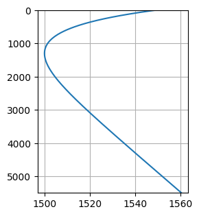
Irregular sound speed profile¶

Preparing environment

[20]:

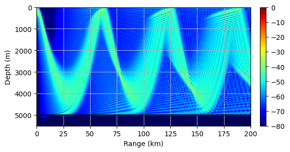
max_range_m = 200E3
env = UnderwaterEnvironment(
    sound_speed_profile_m_s=lambda x, z: munk_profile(z),
    bottom_profile=Bathymetry(ranges_m=[0], depths_m=[5000]),
    bottom_sound_speed_m_s = 1700,
    bottom_density_g_cm = 1.5,
    bottom_attenuation_dm_lambda = 0.5
)

Preparing transmitting antenna

[21]:

src = GaussSource(
    freq_hz=50,
    depth_m=100,
    beam_width_deg=3,
    elevation_angle_deg=0,
    multiplier=5
)

Calculating the acoustics pressure field

[22]:

params = UWASSpadeComputationalParams(
    max_range_m=max_range_m,
    max_depth_m=5500,
    dx_m=100, # output grid steps affects only on the resulting field, NOT the computational grid
    dz_m=5,
)

[23]:

field = uwa_ss_pade(
    src=src,
    env=env,
    params=params
)

Visualising the results

Two dimensional distribution of the field amplitude

[24]:

vis = AcousticPressureFieldVisualiser2d(field=field, env=env)

Munk profile

[25]:

vis.sound_speed_profile().show()

[26]:

vis.plot2d(min_val=-80, max_val=0, grid=True, show_terrain=True).show()

Irregular bottom

[27]:

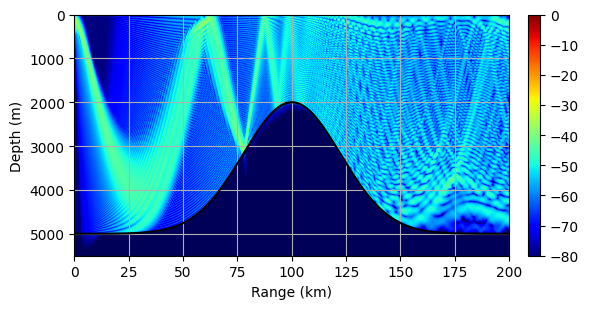
env = UnderwaterEnvironment(
    sound_speed_profile_m_s=lambda x, z: munk_profile(z),
    bottom_profile=Bathymetry(func=lambda z: 5000 - fm.exp((-(z-100E3)**2)/1E9)*3000, max_depth=5000),
    bottom_sound_speed_m_s = 1700,
    bottom_density_g_cm = 1.5,
    bottom_attenuation_dm_lambda = 0.5
)

[28]:

field = uwa_ss_pade(
    src=src,
    env=env,
    params=params
)

[29]:

vis = AcousticPressureFieldVisualiser2d(field=field, env=env)
vis.plot2d(min_val=-80, max_val=0, grid=True, show_terrain=True).show()

[29]: